Chapter 6 Model-based class
All the classes with complex models are grouped into this section.
6.1 trans_diff class
Differential abundance test is an important part in the microbiome profiling analysis.
It can find the significant taxa in determining community differences across groups.
Different approaches may produce inconsistent results since the underlying models/hypothesis are different (Nearing et al. 2022).
Currently, trans_diff class has multiple famous differential test approaches or wrapped methods to better capture the important biomarkers:
Kruskal-Wallis Rank Sum Test (for groups > 2), Wilcoxon Rank Sum Tests (for each paired group),
Dunn’s Kruskal-Wallis Multiple Comparisons (for paired group in cases groups > 2),
t-test, ANOVA, Scheirer Ray Hare test, linear regression,
metastat(White et al. 2009), LEfSe(Segata et al. 2011), RF (random forest + differential test), metagenomeSeq(Paulson et al. 2013),
DESeq2 (Michael I. Love et al. 2014a), ALDEx2 (Fernandes et al. 2014),
ANCOM-BC2 (Lin and Peddada 2020),
LinDA (Zhou et al. 2022), beta regression (Cribari-Neto and Zeileis 2010),
linear mixed-effects model and generalized linear mixed model.
Given that multiple approaches are available,
it is feasible to compare the results from different approaches and extract a part of biomarkers with high confidence for a specific dataset.
![]() Note: The methods for invoking
Note: The methods for invoking otu_table are primarily designed for differential abundance analysis of ASVs/OTUs (or Genes).
These methods for invoking taxa_abund list are recommended for analyses at higher taxonomic levels (such as Genus or Phylum).
6.1.1 Example
All the differential test result is stored in the object$res_diff.
LEfSe combines the non-parametric test and linear discriminant analysis (Segata et al. 2011).
t1 <- trans_diff$new(dataset = mt, method = "lefse", group = "Group", alpha = 0.01, lefse_subgroup = NULL)
# see t1$res_diff for the result
# From v0.8.0, threshold is used for the LDA score selection.
t1$plot_diff_bar(threshold = 4)
# we show 20 taxa with the highest LDA (log10)
t1$plot_diff_bar(use_number = 1:30, width = 0.8, group_order = c("CW", "IW", "TW"))![]()
| Taxa | Group | LDA | P.adj |
|---|---|---|---|
| k__Bacteria|p__Proteobacteria | CW | 4.837 | 1.076e-09 |
| k__Bacteria|p__Acidobacteria | IW | 4.797 | 2.955e-10 |
| k__Bacteria|p__Acidobacteria|c__Acidobacteria | IW | 4.797 | 6.946e-11 |
| k__Bacteria|p__Bacteroidetes | TW | 4.782 | 1.529e-08 |
| k__Bacteria|p__Proteobacteria|c__Gammaproteobacteria | CW | 4.613 | 2.911e-10 |
Then, the abundance of biomarkers detected by LEfSe can be visualized easily.
t1$plot_diff_abund(use_number = 1:30)
t1$plot_diff_abund(fill = "Group", alpha = 0.5, add_sig = FALSE)
t1$plot_diff_abund(group_order = c("CW", "IW", "TW"))
t1$plot_diff_abund(coord_flip = FALSE)
t1$plot_diff_abund(plot_type = "errorbar")
t1$plot_diff_abund(plot_type = "barerrorbar", coord_flip = FALSE)
t1$plot_diff_abund(plot_type = "barerrorbar", errorbar_addpoint = FALSE, errorbar_color_black = TRUE, plot_SE = TRUE)
t1$plot_diff_abund(plot_type = "ggviolin", coord_flip = FALSE)![]()
Then, we show the cladogram of the differential features in the taxonomic tree.
There are too many taxa in this dataset.
As an example, we only select the highest 200 abundant taxa in the tree and 50 differential features.
We only show the full taxonomic label at Phylum level and use letters at other levels to reduce the text overlap.
Note that if an error occurs in this function, the reason with a high probability is the chaotic taxonomy in the user’s data.
Please use the tidy_taxonomy function to solve this issue.
For the tidy_taxonomy examples, please refer to another section (https://chiliubio.github.io/microeco_tutorial/other-examples-1.html#tidy_taxonomy-function).
# clade_label_level 5 represent phylum level in this analysis
# require ggtree package
t1$plot_diff_cladogram(use_taxa_num = 200, use_feature_num = 50, clade_label_level = 5, group_order = c("CW", "IW", "TW"))![]()
There may be a problem related with the taxonomic labels in the plot. When there are too many levels shown, the taxonomic labels can have too much overlap. However, if only Phylum labels are indicated, the taxa in the legend with marked letters are too many. At this time, taxa can be manually choosed to show like the following operation.
# choose some taxa according to the positions in the previous picture; those taxa labels have minimum overlap
tmp <- c("c__Deltaproteobacteria", "c__Actinobacteria", "o__Rhizobiales", "p__Proteobacteria", "p__Bacteroidetes",
    "o__Micrococcales", "p__Acidobacteria", "p__Verrucomicrobia", "p__Firmicutes",
    "p__Chloroflexi", "c__Acidobacteria", "c__Gammaproteobacteria", "c__Betaproteobacteria", "c__KD4-96",
    "c__Bacilli", "o__Gemmatimonadales", "f__Gemmatimonadaceae", "o__Bacillales", "o__Rhodobacterales")
# then use parameter select_show_labels to show
t1$plot_diff_cladogram(use_taxa_num = 200, use_feature_num = 50, select_show_labels = tmp)
# Now we can see that more taxa names appear in the tree![]()
The ‘rf’ method depends on the random forest(Beck and Foster 2014; Yatsunenko et al. 2012) and the non-parametric test. The current method implements random forest by bootstrapping like the operation in LEfSe and employs the significant features as input. MeanDecreaseGini is selected as the indicator value in the analysis.
# use Genus level for parameter taxa_level, if you want to use all taxa, change to "all"
# nresam = 1 and boots = 1 represent no bootstrapping and use all samples directly
t1 <- trans_diff$new(dataset = mt, method = "rf", group = "Group", taxa_level = "Genus")
# plot the MeanDecreaseGini bar
# group_order is designed to sort the groups
g1 <- t1$plot_diff_bar(use_number = 1:20, group_order = c("TW", "CW", "IW"))
# plot the abundance using same taxa in g1
g2 <- t1$plot_diff_abund(group_order = c("TW", "CW", "IW"), select_taxa = t1$plot_diff_bar_taxa, plot_type = "barerrorbar", add_sig = FALSE, errorbar_addpoint = FALSE, errorbar_color_black = TRUE)
# now the y axis in g1 and g2 is same, so we can merge them
# remove g1 legend; remove g2 y axis text and ticks
g1 <- g1 + theme(legend.position = "none")
g2 <- g2 + theme(axis.text.y = element_blank(), axis.ticks.y = element_blank(), panel.border = element_blank())
p <- g1 %>% aplot::insert_right(g2)
p![]()
The significance label can also be added in the abundance plot controlled by add_sig parameter and other related parameters.
Now adding labels supports all the differential test methods.
t1 <- trans_diff$new(dataset = mt, method = "wilcox", group = "Group", taxa_level = "Genus", filter_thres = 0.001)
# filter something not needed to show
t1$res_diff %<>% subset(Significance %in% "***")
t1$plot_diff_abund()
# y_start and y_increase control the position of labels; for the details, please see the document of plot_alpha function in trans_alpha class
t1$plot_diff_abund(y_start = 0.05, y_increase = 0.1)![]()
t1 <- trans_diff$new(dataset = mt, method = "anova", group = "Group", taxa_level = "Genus", filter_thres = 0.001)
t1$plot_diff_abund(coord_flip = F, plot_type = "barerrorbar", errorbar_addpoint = FALSE)![]()
Metastat depends on the permutations and t-test and performs well on the sparse data for paired groups test.
# metastat analysis at Genus level
t1 <- trans_diff$new(dataset = mt, method = "metastat", group = "Group", taxa_level = "Genus")
# t1$res_diff is the differential test result
t1$plot_diff_abund(use_number = 1:20, coord_flip = F)
The following are some examples for the methods ‘KW’, ‘KW_dunn’, ‘wilcox’, ‘t.test’ and ‘anova’.
# Kruskal-Wallis Rank Sum Test for all groups (>= 2)
t1 <- trans_diff$new(dataset = mt, method = "KW", group = "Group", taxa_level = "all", filter_thres = 0.001)
t1$plot_diff_abund(use_number = 1:20)
# Dunn's Kruskal-Wallis Multiple Comparisons when group number > 2; require FSA package
t1 <- trans_diff$new(dataset = mt, method = "KW_dunn", group = "Group", taxa_level = "Genus", filter_thres = 0.0001)
t1$plot_diff_abund(use_number = 1:10, add_sig = T, coord_flip = F)
# Wilcoxon Rank Sum and Signed Rank Tests for all paired groups
t1 <- trans_diff$new(dataset = mt, method = "wilcox", group = "Group", taxa_level = "Genus", filter_thres = 0.001)
t1$plot_diff_bar(use_number = 1:20)
t1$plot_diff_abund(use_number = 1:20)
# t.test
t1 <- trans_diff$new(dataset = mt, method = "t.test", group = "Group", taxa_level = "all", filter_thres = 0.001)
# anova
t1 <- trans_diff$new(dataset = mt, method = "anova", group = "Group", taxa_level = "Phylum", filter_thres = 0.001)
head(t1$res_diff)
The method ‘metagenomeSeq’ (Paulson et al. 2013) and ‘ancombc2’ (Lin and Peddada 2020) depend on the metagenomeSeq package and ANCOMBC package, respectively. The method ‘ALDEx2_t’ and ‘ALDEx2_kw’ depend on the ALDEx2 package (Fernandes et al. 2014). These three packages are all deposited on the Bioconductor.
# zero-inflated log-normal model-based differential test method from metagenomeSeq package
# If metagenomeSeq package is not installed, please first run: BiocManager::install("metagenomeSeq")
t1 <- trans_diff$new(dataset = mt, method = "metagenomeSeq", group = "Group", taxa_level = "OTU")
t1$plot_diff_abund(use_number = 1:30, group_order = c("TW", "CW", "IW"))
t1$plot_diff_bar(use_number = 1:20)
t1$plot_volcano()
t1$plot_volcano(select_group = 2)
# 'ALDEx2_t' and 'ALDEx2_kw' methods; use ?trans_diff to see detailed description of the methods
# If ALDEx2 package is not installed, please first run: BiocManager::install("ALDEx2")
# 'ALDEx2_t'
t1 <- trans_diff$new(dataset = mt, method = "ALDEx2_t", group = "Group", taxa_level = "OTU", filter_thres = 0.0005)
t1$plot_diff_abund()
# ALDEx2_kw
t1 <- trans_diff$new(dataset = mt, method = "ALDEx2_kw", group = "Group", taxa_level = "OTU", filter_thres = 0.001)
t1$plot_diff_abund(use_number = 1:30, group_order = c("TW", "CW", "IW"))
t1$plot_diff_bar(use_number = 1:20)
t1$plot_diff_abund(use_number = 1:30, group_order = c("TW", "CW", "IW"), add_sig = TRUE)# ANCOMBC2 method
# when fix_formula is not provided (necessary in ancombc2 function of ANCOMBC package), it will be assigned automatically by using group parameter
# Restart R if there is an error that "Error in model.matrix.formula(): data must be a data.frame"
t1 <- trans_diff$new(dataset = mt, method = "ancombc2", group = "Group", taxa_level = "OTU", filter_thres = 0.01)
t1$plot_diff_bar(keep_full_name = TRUE, heatmap_cell = "P.adj", heatmap_sig = "Significance", heatmap_x = "Factors", heatmap_y = "Taxa")
# add a continuous variable
tmp <- clone(mt)
tmp$sample_table <- data.frame(tmp$sample_table, env_data_16S[rownames(tmp$sample_table), ])
t2 <- trans_diff$new(dataset = tmp, method = "ancombc2", group = NULL, fix_formula = "pH+Group", taxa_level = "OTU", filter_thres = 0.005)
# original results t2$res_diff_raw
# converted result t2$res_diff
View(t2$res_diff)The method linda (Zhou et al. 2022) depends on the MicrobiomeStat package.
# LinDA method. If MicrobiomeStat package is not installed, please first run: install.packages("MicrobiomeStat")
t1 <- trans_diff$new(dataset = mt, method = "linda", group = "Group", taxa_level = "OTU", filter_thres = 0.001)
t1$plot_diff_abund(use_number = 1:30, group_order = c("TW", "CW", "IW"), add_sig = TRUE)
View(t1$res_diff)
t1$plot_diff_bar(keep_full_name = TRUE)
# Either group or formula parameter should be provided in v1.5.0. Then are same for linda method.
tmp <- clone(mt)
tmp$sample_table <- data.frame(tmp$sample_table, env_data_16S[rownames(tmp$sample_table), ])
t1 <- trans_diff$new(dataset = tmp, method = "linda", group = "pH + Group", taxa_level = "OTU", filter_thres = 0.001)
t2 <- trans_diff$new(dataset = tmp, method = "linda", formula = "~pH + Group", taxa_level = "OTU", filter_thres = 0.001)
t2$plot_diff_bar(keep_full_name = FALSE, color_values = c("#053061", "white", "#A50026"), trans = "log10", filter_feature = "", ytext_position = "left")
6.1.2 More options
The dependence packages in the following examples are not mentioned in the previous package dependence part (https://chiliubio.github.io/microeco_tutorial/intro.html#dependence).
The methods DESeq2 and edgeR are also supported in the trans_diff class and no longer demonstrated here.
The linear regression from lm function and linear mixed-effects models from lmerTest package can be fitted with the option method = 'lm' and method = 'lme', respectively.
The heatmap can be used in the plot_diff_bar function instead of bar plot for the case with multiple factors or formula.
# AST: arc sine square root transformation
if(!require("lmerTest")) install.packages("lmerTest")
t1 <- trans_diff$new(dataset = mt, method = "lme", formula = "Group+(1|Type)", taxa_level = "Phylum", transformation = "AST", filter_thres = 0.001)
View(t1$res_diff)
t1$plot_diff_bar(heatmap_cell = "Estimate", heatmap_sig = "Significance", heatmap_lab_fill = "Coefficient")
The generalized linear mixed model (GLMM) is implemented based on the glmmTMB package. In this example, we use beta distribution function as the family function, because beta distribution is especially appropriate to fit the proportional data (relative abundance here). When no random effects are present, the ‘glmm_beta’ method is equivalent to the ‘betareg’ method (beta regression).
if(!require("glmmTMB")) install.packages("glmmTMB")
tmp <- clone(mt)
t1 <- trans_diff$new(dataset = tmp, taxa_level = "Phylum", method = "glmm_beta",
    formula = "Group + (1|Type)", filter_thres = 0.001)
View(t1$res_diff)
t1$plot_diff_bar(heatmap_cell = "Estimate", heatmap_sig = "Significance", heatmap_lab_fill = "Coefficient")
Let’s run two-way anova for more usages of heatmap.
t1 <- trans_diff$new(dataset = mt, method = "anova", formula = "Group + Type", taxa_level = "Phylum", filter_thres = 0.001, transformation = "AST")
t1$plot_diff_bar()
t1$plot_diff_bar(color_palette = rev(RColorBrewer::brewer.pal(n = 11, name = "RdYlBu")), trans = "log10")
t1$plot_diff_bar(color_values = c("#053061", "white", "#A50026"), trans = "log10")
t1$plot_diff_bar(color_values = c("#053061", "white", "#A50026"), trans = "log10", filter_feature = "", ytext_position = "right", cluster_ggplot = "row")
6.1.3 Key points
- trans_diff$new: In trans_diff$new, p_adjust_method = “none” can close the p value adjustment. This is useful in cases where very few significant taxa are found (generally no significant feature found after adjustment) and where LEfSe result is needed to be compared with that from Galaxy server or other LEfSe python version.
- trans_diff$new: this class has a strict requirement on the taxonomic information,
make sure
tidy_taxonomy()function has been performed for thetax_tableinmicrotableobject. - trans_diff$new: creating this class invokes one or more tables in
taxa_abundlist, which is stored inmicrotableobject. - trans_diff$plot_diff_cladogram:
clade_label_size,clade_label_size_addandclade_label_size_logcan control the text size all together in the cladogram. - trans_diff$new: from v0.19.0,
transformationparameter can be employed to transform or normalize relative abundance data based on the mecodev package for those methods coming from trans_alpha class (“KW”, “KW_dunn”, “wilcox”, “t.test”, “anova”, “scheirerRayHare”, “betareg”, “lme”, “glmm”). For example,transformation = 'AST'represents the arc sine square root transformation. - trans_diff$plot_diff_bar: from v0.19.0,
color_group_map = TRUEcan be added inplot_diff_barfunction to fix the color in each group when part of groups are not shown in the plot, which is especially useful when multiple approaches or data are needed to run the same step.
6.2 trans_network class
Network analysis has been frequently used to study microbial co-occurrence patterns (Deng et al. 2012; Faust and Raes 2012; Coyte et al. 2015). In this part, we describe part of the implemented methods in the trans_network class.

The objects inside the rectangle with full line represent functions.
The dashed line denotes the key objects (input or output). The res_network inside the ellipse with dashed line means it is a hub object for other analysis.
6.2.1 Example
The correlation-based network is selected to show the main operations. This is only intended to show some operations conveniently. Do not mean we are suggesting this approach in any case. Please check the final part for other network construction methods.
# The parameter cor_method in trans_network is used to select correlation calculation method.
# default pearson or spearman correlation invoke R base cor.test, a little slow
t1 <- trans_network$new(dataset = mt, cor_method = "spearman", filter_thres = 0.001)
# return t1$res_cor_p list, containing two tables: correlation coefficient table and p value table
Spearman correlation based on WGCNA package is applied to show all the following operations.
# require WGCNA package
if(!require("WGCNA")) install.packages("WGCNA", repos = BiocManager::repositories())
t1 <- trans_network$new(dataset = mt, cor_method = "spearman", use_WGCNA_pearson_spearman = TRUE, filter_thres = 0.0001)
The parameter COR_cut can be used to select the correlation threshold.
Furthermore, COR_optimization = TRUE can be used to find the optimized coefficient threshold (potential transition point of network eigenvalues)
instead of the COR_cut based on the RMT theory (Deng et al. 2012).
# construct network; require igraph package
t1$cal_network(COR_p_thres = 0.01, COR_optimization = TRUE)
# use arbitrary coefficient threshold to contruct network
t1$cal_network(COR_p_thres = 0.01, COR_cut = 0.7)
# return t1$res_network
Then, let’s partition modules for the network.
# invoke igraph cluster_fast_greedy function for this undirected network
t1$cal_module(method = "cluster_fast_greedy")
The following operation is to save network to gexf format for the visualization with Gephi(https://gephi.org/). The file ‘network.gexf’ can be directly opened by Gephi.
Then, we plot the network in Gephi and present the node colors according to the partitioned modules.
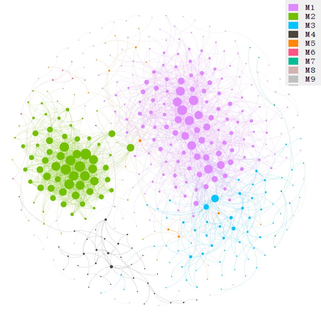
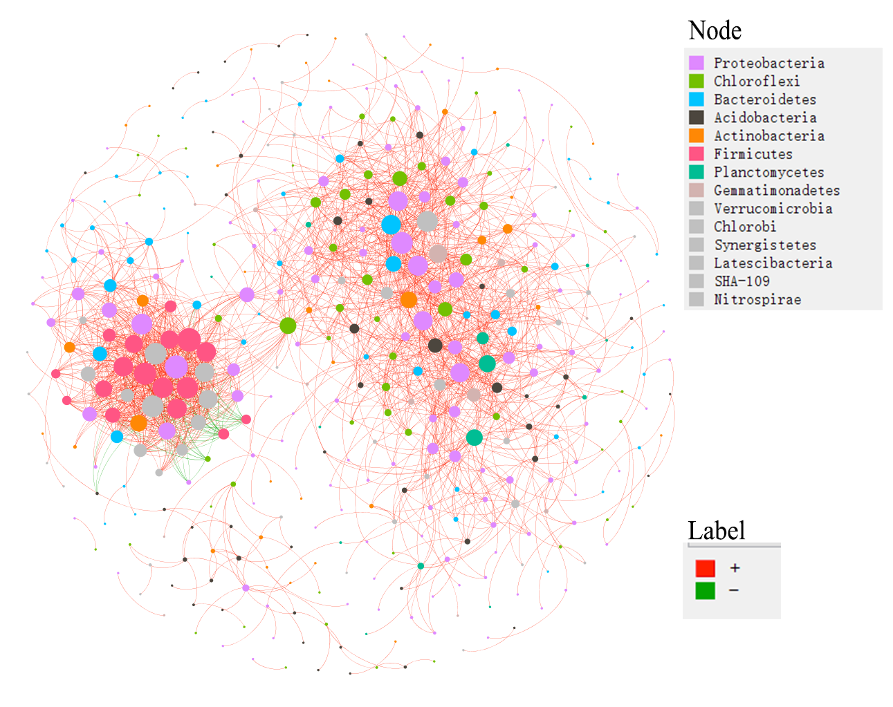
Now, we show the node colors with the Phylum information and the edges colors with the positive and negative correlations. All the data used has been stored in the network.gexf file, including modules classifications, Phylum information and edge labels.
| Property | Value |
|---|---|
| Vertex | 407 |
| Edge | 1989 |
| Average_degree | 9.774 |
| Average_path_length | 3.878 |
| Network_diameter | 9 |
| Clustering_coefficient | 0.4698 |
| Density | 0.02407 |
| Heterogeneity | 1.194 |
| Centralization | 0.09908 |
The function get_node_table, get_edge_table and get_adjacency_matrix are designed to get node properties table, edge properties table and adjacency matrix from network, respectively.
| name | degree | betweenness | Abundance | module | z | |
|---|---|---|---|---|---|---|
| OTU_50 | OTU_50 | 2 | 0 | 0.2301 | M2 | -1.305 |
| OTU_305 | OTU_305 | 3 | 4 | 0.1394 | M8 | 1.118 |
| OTU_1 | OTU_1 | 21 | 2 | 1.409 | M2 | -0.04067 |
| OTU_41 | OTU_41 | 1 | 0 | 0.1603 | M14 | -0.5774 |
| OTU_59 | OTU_59 | 3 | 2306 | 0.5588 | M6 | 0.7771 |
# get edge properties
t1$get_edge_table()
# return t1$res_edge_table
t1$get_adjacency_matrix()
# return t1$res_adjacency_matrix
Then, let’s plot the node classification in terms of the within-module connectivity and among-module connectivity.
# add_label = TRUE can be used to directly add text label for points
t1$plot_taxa_roles(use_type = 1)![]()
![]()
Now, we show the eigengene analysis of modules. The eigengene of a module, i.e. the first principal component of PCA, represents the main variance of the abundance in the species of the module.
Then we perform correlation heatmap to show the associations between eigengenes and environmental factors.
# create trans_env object
t2 <- trans_env$new(dataset = mt, add_data = env_data_16S[, 4:11])
# calculate correlations
t2$cal_cor(add_abund_table = t1$res_eigen)
# plot the correlation heatmap
t2$plot_cor()![]()
The subset_network function can be applied to extract a part of nodes and edges among these nodes from the network.
In this function, you should provide the nodes you need using the node parameter.
# extract a sub network that contains all nodes in module M1
t1$subset_network(node = t1$res_node_table %>% base::subset(module == "M1") %>% rownames, rm_single = TRUE)
# return a new network with igraph class
# extract sub network in which all edge labels are "+", i.e. positive edges
t1$subset_network(edge = "+")
Then let’s show how to extract sub-network for samples (Ma et al. 2016).
# extract the sub-network of sample 'S1'
sub1 <- t1$subset_network(sample_name = "S1", return_igraph = FALSE)
# return_igraph = FALSE means return is trans_network object instead of igraph object
sub1$cal_module()
sub1$save_network("S1.gexf")
Extract all sub-networks for each sample.
samples_network <- list()
for(i in rownames(t1$data_abund)){
    samples_network[[i]] <- t1$subset_network(return_igraph = FALSE, sample_name = i)
}
# when return_igraph = FALSE, samples_network can be the input for functions in meconetcomp package
We also add the function plot_network to directly plot the network in R, including the static network and dynamic network.
The static network is suitable for the case with relatively few nodes, while dynamic network can be better applied to a large network.
See https://yunranchen.github.io/intro-net-r/advanced-network-visualization.html and https://kateto.net/network-visualization for more
details on the network visualization in R.
# default parameter represents using igraph plot.igraph function
t2$plot_network()
# use ggraph method; require ggraph package
# If ggraph is not installed; first install it with command: install.packages("ggraph")
t2$plot_network(method = "ggraph", node_color = "Phylum")
# use networkD3 package method for the dynamic network visualization in R
# If networkD3 is not installed; first install it with command: install.packages("networkD3")
t1$plot_network(method = "networkD3", node_color = "module")
t1$plot_network(method = "networkD3", node_color = "Phylum")
The trans_comm function can be used to convert the node classification to a new microtable object for other analysis.
# use_col is used to select a column of t1$res_node_table
tmp <- t1$trans_comm(use_col = "module", abundance = FALSE)
tmp
tmp$otu_table[tmp$otu_table > 0] <- 1
tmp$tidy_dataset()
tmp$cal_abund()
tmp2 <- trans_abund$new(tmp, taxrank = "Phylum", ntaxa = 10)
tmp2$data_abund$Sample %<>% factor(., levels = rownames(tmp$sample_table))
tmp2$plot_line(xtext_angle = 30, color_values = RColorBrewer::brewer.pal(12, "Paired")) + ylab("OTUs ratio (%)")
The function cal_sum_links can sum the links (edge) number from one taxa to another or within the same taxa.
The function plot_sum_links is used to show the result from the function cal_sum_links.
This is very useful to fast see how many nodes are connected between different taxa or within one taxa.
In terms of ‘Phylum’ level in the tutorial, the function cal_sum_links() sum the linkages number from one Phylum to another Phylum or the linkages in the same Phylum.
So the numbers along the outside of the circular plot represent how many edges or linkages are related with the Phylum.
For example, in terms of Proteobacteria, there are roughly total 900 edges associated with the OTUs in Proteobacteria,
in which roughly 200 edges connect both OTUs in Proteobacteria and roughly 150 edges connect the OTUs from Proteobacteria with the OTUs from Chloroflexi.
t1$cal_sum_links(taxa_level = "Phylum")
# interactive visualization; require chorddiag package; see https://github.com/mattflor/chorddiag
t1$plot_sum_links(plot_pos = TRUE, plot_num = 10, color_values = RColorBrewer::brewer.pal(10, "Paired"))
# From v1.2.0, method = "circlize" is available for conveniently saving the static plot
# If circlize package is not installed, first run: install.packages("circlize")
t1$plot_sum_links(method = "circlize", transparency = 0.2, annotationTrackHeight = circlize::mm_h(c(5, 5)))![]()
For the correlation network, there are also other available correlation/association calculation options, such as Bray–Curtis (1-dissimilarity), SparCC (Friedman and Alm 2012), CCLasso (Fang et al. 2015), Pearson or Spearman with data normalization based on NetCoMi package (Peschel et al. 2021).
# use Bray–Curtis index (1-dissimilarity)
t1 <- trans_network$new(dataset = mt, cor_method = "bray", filter_thres = 0.001)
# Pearson correlation
t1 <- trans_network$new(dataset = mt, cor_method = "pearson", filter_thres = 0.001)
# Pearson correlation using WGCNA package
# install WGCNA package
if(!require("WGCNA")) install.packages("WGCNA", repos = BiocManager::repositories())
t1 <- trans_network$new(dataset = mt, cor_method = "pearson", use_WGCNA_pearson_spearman = TRUE, filter_thres = 0.001)
# Pearson correlation using NetCoMi package; install it from https://github.com/stefpeschel/NetCoMi
t1 <- trans_network$new(dataset = mt, cor_method = "pearson", use_NetCoMi_pearson_spearman = TRUE, filter_thres = 0.001)
# Spearman correlation using WGCNA package
t1 <- trans_network$new(dataset = mt, cor_method = "spearman", use_WGCNA_pearson_spearman = TRUE, filter_thres = 0.001)
# Spearman correlation using NetCoMi package
t1 <- trans_network$new(dataset = mt, cor_method = "spearman", use_NetCoMi_pearson_spearman = TRUE, filter_thres = 0.001)
# SparCC method, from SpiecEasi package, see https://github.com/zdk123/SpiecEasi for the installation
t1 <- trans_network$new(dataset = mt, cor_method = "sparcc", use_sparcc_method = "SpiecEasi", filter_thres = 0.003)
# SparCC method, from NetCoMi package; https://github.com/stefpeschel/NetCoMi
t1 <- trans_network$new(dataset = mt, cor_method = "sparcc", use_sparcc_method = "NetCoMi", filter_thres = 0.001)
# CCLasso method based on NetCoMi package
t1 <- trans_network$new(dataset = mt, cor_method = "cclasso", filter_thres = 0.001)
# CCREPE method based on NetCoMi package
t1 <- trans_network$new(dataset = mt, cor_method = "ccrepe", filter_thres = 0.001)
Then let’s show other implemented network construction approaches:
SPIEC-EASI (SParse InversE Covariance Estimation for Ecological Association Inference) approach of SpiecEasi R package (Kurtz et al. 2015)
has two network construction approaches based on graph model, which relies on algorithms for sparse neighborhood and inverse covariance selection.
See https://github.com/zdk123/SpiecEasi for the package installation.
It is very slow for SpiecEasi_method = ‘glasso’ when there is a large number (such as hundreds to thousands) according to our test experience.
t1 <- trans_network$new(dataset = mt, cor_method = NULL, taxa_level = "OTU", filter_thres = 0.001)
# require SpiecEasi package installed https://github.com/zdk123/SpiecEasi
# also see SpiecEasi::spiec.easi for available model parameters
t1$cal_network(network_method = "SpiecEasi", SpiecEasi_method = "mb")
# see t1$res_network
Another network construction approach comes from julia package FlashWeave (Tackmann et al. 2019). This is a probabilistic graph-based method to obtain the conditional independence. It predicts direct associations among microbes from large-scale compositional abundance data through statistical co-occurrence. To repeat the following code, please first install julia language in your computer and the FlashWeave package, and add the julia in the computer path.
- download and install julia from https://julialang.org/downloads/
- Put julia in the computer env PATH, such as your_directory_path
- Open terminal or cmd or Powershell, open julia, install FlashWeave following the operation in https://github.com/meringlab/FlashWeave.jl
t1 <- trans_network$new(dataset = mt, cor_method = NULL, taxa_level = "OTU", filter_thres = 0)
# require Julia in the computer path, and the package FlashWeave
# different with the direct parameter passing of 'SpiecEasi' network_method, FlashWeave_other_para is used to pass parameters to Julia FlashWeave
# assign FlashWeave_tempdir parameter can change the temporary working directory
t1$cal_network(network_method = "FlashWeave", FlashWeave_other_para = "alpha=0.01,sensitive=true,heterogeneous=true")
# see t1$res_network
The final method we want to show comes from beemStatic package (Li et al. 2021). This method can be applied to cross-sectional datasets to infer interaction network based on the generalized Lotka-Volterra model, which is typically used in the microbial time-series data. So the network from this approach is a directed network. Please see https://github.com/CSB5/BEEM-static for installing the R beemStatic package.
6.2.2 Network comparison
To compare different networks from trans_network class, please see the meconetcomp package chapter (https://chiliubio.github.io/microeco_tutorial/meconetcomp-package.html).
6.2.3 Key points
- cal_network(): get a network named
res_networkbased on different methods - get_node_table(): get node properties table
- subset_network(): this function can extract any sub-network according to the input nodes, e.g. sub-network for modules or samples
6.2.4 Other functions
- cal_powerlaw(): perform bootstrapping hypothesis test to determine whether degrees follow a power law distribution and fit degrees to a power law distribution.
- random_network(): generate random networks, compare them with the empirical network and get the p value of topological properties.
6.3 trans_nullmodel class
In recent decades, the integration of phylogenetic analysis and null model promotes the inference of niche and neutral influences on community assembly more powerfully by adding a phylogeny dimension (Webb et al. 2002; Kembel et al. 2010; Stegen et al. 2013). The trans_nullmodel class provides an encapsulation, including the calculation of the phylogenetic signal, beta mean pairwise phylogenetic distance (betaMPD), beta mean nearest taxon distance (betaMNTD), beta nearest taxon index (betaNTI), beta net relatedness index (betaNRI) and Bray-Curtis-based Raup-Crick (RCbray). The approach for phylogenetic signal analysis is based on the mantel correlogram (C. Liu et al. 2017), in which the change of phylogenetic signal is intuitional and clear compared to other approaches. The combinations between RCbray and betaNTI can be used to infer the strength of each ecological process dominating the community assembly under the specific hypothesis (Stegen et al. 2013).
6.3.1 Example
We first check the phylogenetic signal.
# generate trans_nullmodel object
# as an example, we only use high abundance OTU with mean relative abundance > 0.0005
t1 <- trans_nullmodel$new(mt, filter_thres = 0.0005, add_data = env_data_16S)
# use pH as the test variable
t1$cal_mantel_corr(use_env = "pH")
# return t1$res_mantel_corr
# plot the mantel correlogram
t1$plot_mantel_corr()![]()
betaNRI(ses.betampd) is used to show the ‘basal’ phylogenetic turnover. Compared to betaNTI, it can capture more turnover information associated with the deep phylogeny. It is noted that there are many null models with the development in the several decades of community ecology. In the trans_nullmodel class, the default null mode of betaNTI and betaNRI is the randomization of the phylogenetic relatedness among species. This shuffling approach fix the observed levels of species α-diversity and β-diversity to explore whether the observed phylogenetic turnover significantly differ from null model that phylogenetic relatedness among species are random.
# see null.model parameter for other null models
# null model run 500 times for the example
t1$cal_ses_betampd(runs = 500, abundance.weighted = TRUE)
# return t1$res_ses_betampd
If we want to plot the betaNRI, we can use plot_group_distance function in trans_beta class. For example, the results showed that the mean betaNRI of TW is extremely and significantly larger that those in CW and IW, revealing that the basal phylogenetic turnover in TW is high.
# add betaNRI matrix to beta_diversity list
mt$beta_diversity[["betaNRI"]] <- t1$res_ses_betampd
# create trans_beta class, use measure "betaNRI"
t2 <- trans_beta$new(dataset = mt, group = "Group", measure = "betaNRI")
# transform the distance for each group
t2$cal_group_distance()
# see the help document for more methods, e.g. "anova" and "KW_dunn"
t2$cal_group_distance_diff(method = "wilcox")
# plot the results
g1 <- t2$plot_group_distance(add = "mean")
g1 + geom_hline(yintercept = -2, linetype = 2) + geom_hline(yintercept = 2, linetype = 2)![]()
BetaNTI(ses.betamntd) can be used to indicate the phylogenetic terminal turnover (Stegen et al. 2013).
# null model run 500 times
t1$cal_ses_betamntd(runs = 500, abundance.weighted = TRUE, null.model = "taxa.labels")
# return t1$res_ses_betamntd| S1 | S2 | S3 | S4 | S5 | |
|---|---|---|---|---|---|
| S1 | 0 | -0.432 | -0.7318 | 0.6482 | 1.236 |
| S2 | -0.432 | 0 | -0.9817 | 0.1372 | 0.8991 |
| S3 | -0.7318 | -0.9817 | 0 | 1.098 | 0.02069 |
| S4 | 0.6482 | 0.1372 | 1.098 | 0 | -1.085 |
| S5 | 1.236 | 0.8991 | 0.02069 | -1.085 | 0 |
If the dataset is large, it is faster with use_iCAMP = TRUE for betaNTI.
tmp <- "./test1"; dir.create(tmp)
t1$cal_ses_betamntd(runs = 1000, abundance.weighted = TRUE, use_iCAMP = TRUE, iCAMP_tempdir = tmp)
RCbray (Bray-Curtis-based Raup-Crick) can be calculated using function cal_rcbray() to assess whether the compositional turnover was governed primarily by drift (Chase et al. 2011). We applied null model to simulate species distribution by randomly sampling individuals from each species pool with preserving species occurrence frequency and sample species richness (C. Liu et al. 2017).
As an example, we also calculate the proportion of the inferred processes on the community assembly as shown in the references (Stegen et al. 2013; C. Liu et al. 2017). In the example, the fraction of pairwise comparisons with significant betaNTI values (|βNTI| > 2) is the estimated influence of Selection; βNTI > 2 represents the heterogeneous selection; βNTI < -2 represents the homogeneous selection. The value of RCbray characterizes the magnitude of deviation between observed Bray–Curtis and Bray–Curtis expected under the randomization; a value of |RCbray| > 0.95 was considered significant. The fraction of all pairwise comparisons with |βNTI| < 2 and RCbray > +0.95 was taken as the influence of Dispersal Limitation combined with Drift. The fraction of all pairwise comparisons with |βNTI| < 2 and RCbray < -0.95 was taken as an estimate for the influence of Homogenizing Dispersal. The fraction of all pairwise comparisons with |βNTI| < 2 and |RCbray| < 0.95 estimates the influence of Drift acting alone.
## The result is stored in object$res_process ...## The result is stored in object$res_process ...| process | percentage |
|---|---|
| variable selection | 9.238 |
| homogeneous selection | 0 |
| dispersal limitation | 8.964 |
| homogeneous dispersal | 11.54 |
| drift | 70.26 |
The cal_NST function can be used to calculate normalized stochasticity ratio based on the NST package (Ning et al. 2019),
including ‘tNST’ and ‘pNST’ methods.
# require NST package to be installed
t1$cal_NST(method = "tNST", group = "Group", dist.method = "bray", abundance.weighted = TRUE, output.rand = TRUE, SES = TRUE)
t1$res_NST$index.grp
## Perform tNST analysis ...## All match very well.## Now randomizing by parallel computing. Begin at Wed Jul 15 14:16:16 2026. Please wait...## The result is stored in object$res_NST ...| group | size | ST.i.bray | NST.i.bray | MST.i.bray | SES.i.bray |
|---|---|---|---|---|---|
| IW | 435 | 0.555 | 0.2909 | 0.3006 | 19.9 |
| CW | 435 | 0.5886 | 0.3141 | 0.3179 | 24.31 |
| TW | 435 | 0.5824 | 0.3602 | 0.3669 | 17.23 |
# convert long format table to square matrix
# the 10th column: MST.ij.bray in t1$res_NST$index.pair
test <- t1$cal_NST_convert(10)
# for pNST method, phylogenetic tree is needed
t1$cal_NST(method = "pNST", group = "Group", output.rand = TRUE, SES = TRUE)
t1$cal_NST_test(method = "nst.boot")For nearest Taxon Index (NTI) and nearest Relative Index (NRI), please use cal_NTI and cal_NRI, respectively.
6.4 trans_classifier class
The trans_classifier class is a wrapper for methods of machine-learning-based classification models. Microbiome-based supervised machine-learning has been successful in predicting human health status (Poore et al. 2020) and soil categories (Wilhelm et al. 2021).
6.4.2 Examples
In this section, we use the example data in file2meco package (https://chiliubio.github.io/microeco_tutorial/file2meco-package.html) to demonstrate the feature selection, data training and prediction with random forest algorithm.
library(microeco)
library(file2meco)
abund_file_path <- system.file("extdata", "dada2_table.qza", package="file2meco")
sample_file_path <- system.file("extdata", "sample-metadata.tsv", package="file2meco")
taxonomy_file_path <- system.file("extdata", "taxonomy.qza", package="file2meco")
# construct microtable object
d1 <- qiime2meco(feature_table = abund_file_path, sample_table = sample_file_path, taxonomy_table = taxonomy_file_path)
d1$cal_abund()

# initialize: use "genotype" as response variable
# x.predictors parameter is used to select the taxa; here we use all the taxa data in d1$taxa_abund
t1 <- trans_classifier$new(dataset = d1, y.response = "genotype", x.predictors = "All")
We silit the data into training and testing set.
Before training the model, we run the set_trainControl to invoke the trainControl function of caret package to generate the parameters used for training. Here we use the default parameters in trainControl function.
Now let’s start model training with rf method.
We can use cal_predict function to predict the testing data set.
Using cal_ROC and plot_ROC can get the ROC (Receiver Operator Characteristic) curve.
t1$cal_ROC()
# select one group to plot ROC
t1$plot_ROC(plot_group = "susceptible")
t1$plot_ROC(plot_group = "susceptible", color_values = "black")
# default all groups
t1$plot_ROC(size = 0.5, alpha = 0.7)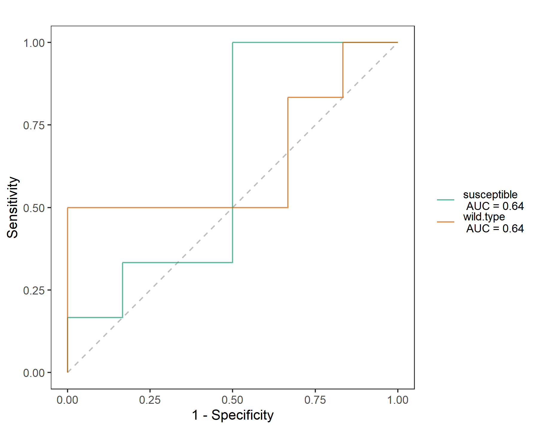
While building a machine learning model for microbiome data, the huge diversity of microbial community and/or associated relationships among taxa accross phylogeny can lead to a large number of unnecessary features, which can reduce the overall accuracy, increase the complexity and overfit of the model and decrease the generalization capability of the model. So, feature selection is one important step in building machine-learning model. Then, we attempt to use Boruta package (Kursa and Rudnicki 2010) to do feature selection.
To compare the results between the procedure with feature selection and that without feature selection, we also perfom all the analysis with feature selection to show the whole results.
t2 <- trans_classifier$new(dataset = d1, y.response = "genotype", x.predictors = "All")
t2$cal_split(prop.train = 3/4)
t2$cal_feature_sel(boruta.maxRuns = 300, boruta.pValue = 0.01)
t2$set_trainControl()
t2$cal_train()
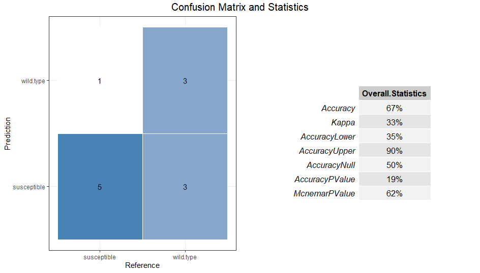
t2$cal_predict()
t2$plot_confusionMatrix()
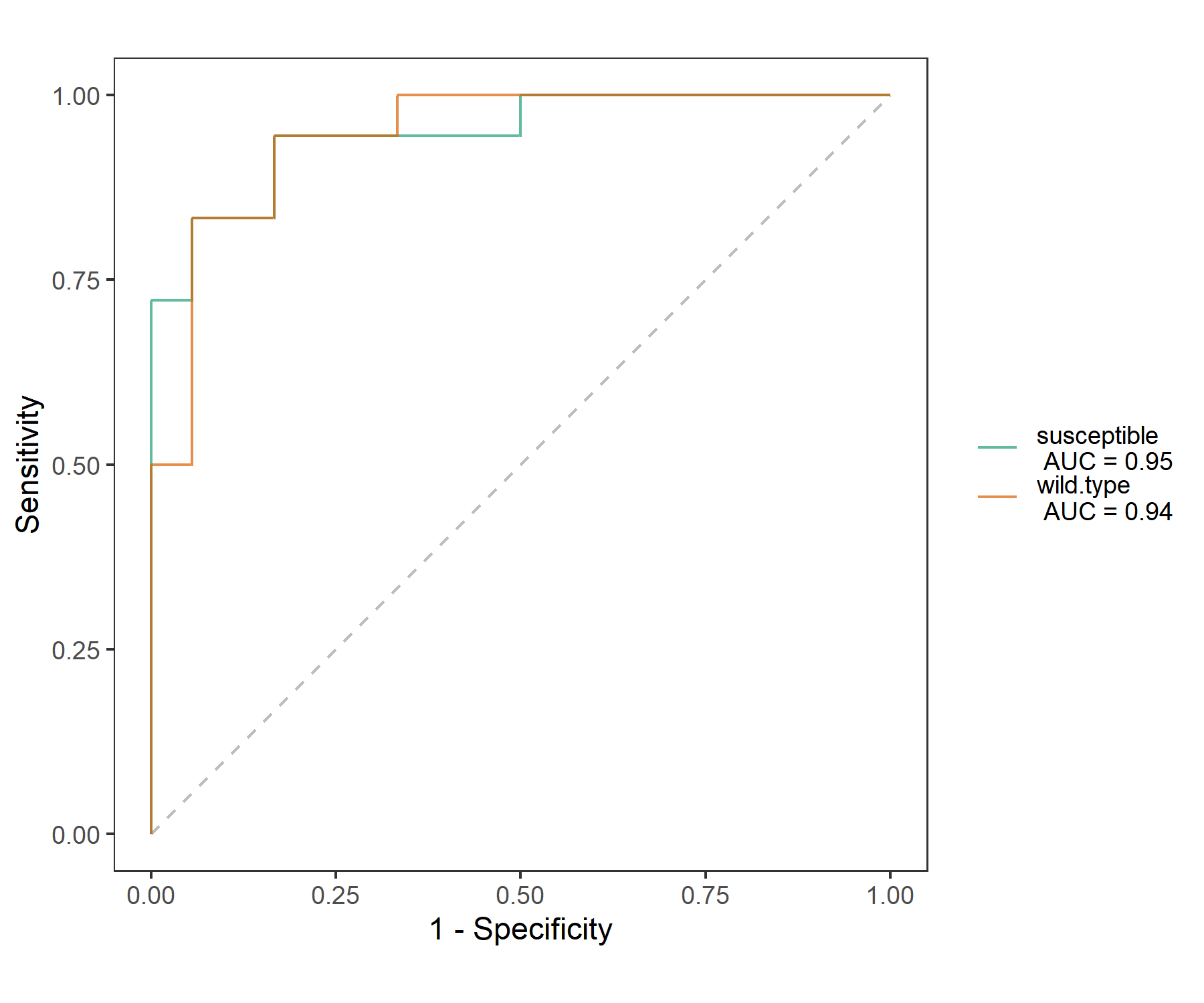
t2$cal_ROC()
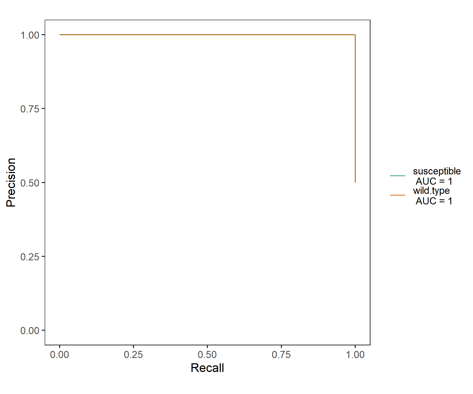
t2$plot_ROC(size = 0.5, alpha = 0.7)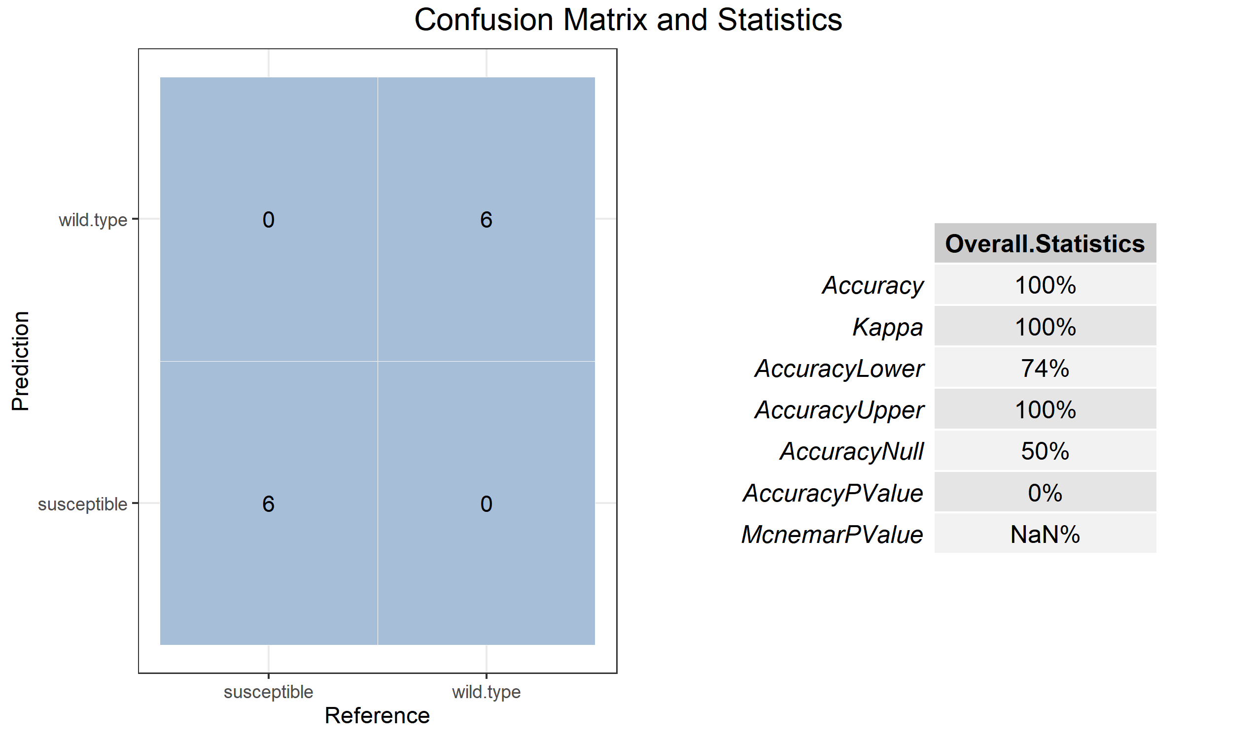

To plot the Precision-Recall curve (PR curve), please make plot_type = “PR” in plot_ROC function.
To show the ROC curve or PR curve of the training result, please make input = “train” in plot_ROC function.
To obtain the feature importance, please use cal_feature_imp function.
# default method in caret package without significance
t2$cal_feature_imp()
t2$plot_feature_imp(colour = "red", fill = "red", width = 0.6)
# generate significance with rfPermute package
t2$cal_feature_imp(rf_feature_sig = TRUE, num.rep = 1000)
# add_sig = TRUE: add significance label
t2$plot_feature_imp(coord_flip = FALSE, colour = "red", fill = "red", width = 0.6, add_sig = TRUE)
# show_sig_group = TRUE: show different colors in groups with different significance labels
t2$plot_feature_imp(show_sig_group = TRUE, coord_flip = FALSE, width = 0.6, add_sig = TRUE)
t2$plot_feature_imp(show_sig_group = TRUE, coord_flip = TRUE, width = 0.6, add_sig = TRUE)
# rf_sig_show = "MeanDecreaseGini": switch to MeanDecreaseGini
t2$plot_feature_imp(show_sig_group = TRUE, rf_sig_show = "MeanDecreaseGini", coord_flip = TRUE, width = 0.6, add_sig = TRUE)
# group_aggre = FALSE: donot aggregate features for each group
t2$plot_feature_imp(show_sig_group = TRUE, rf_sig_show = "MeanDecreaseGini", coord_flip = TRUE, width = 0.6, add_sig = TRUE, group_aggre = FALSE)
For other machine-learning models, please use method parameter in cal_train function.
The regression is also supported.
# prepare data
data(env_data_16S)
tmp <- clone(mt)
tmp$sample_table <- data.frame(tmp$sample_table, env_data_16S[rownames(tmp$sample_table), ])
# pH response variable
t1 <- trans_classifier$new(dataset = tmp, y.response = "pH", x.predictors = "Genus")
t1$cal_split(prop.train = 3/4)
# optional: preprocessing
# t1$cal_preProcess(method = c("center", "scale"))
t1$set_trainControl()
t1$cal_train()
t1$res_train
t1$cal_predict()
t1$res_predict
# feature importance
t1$cal_feature_imp()
head(t1$res_feature_imp)
t1$plot_feature_imp(use_number = 1:20) + ylab("IncNodePurity")

# sort and select some taxa with high importance
tmp_top20 <- rownames(t1$res_feature_imp[order(t1$res_feature_imp[, 1], decreasing = TRUE), , drop = FALSE])[1:20]
# correlation analysis
t2 <- trans_env$new(dataset = tmp, add_data = env_data_16S[, 4:11])
t2$cal_cor(use_data = "other", other_taxa = gsub("`", "", tmp_top20))
t2$plot_cor()