Chapter 7 Explainable class
The trans_env and trans_func classes are placed into the section ‘Explainable class’, as environmental factors, microbial functions and metabolites can be generally applied to explain microbial dynamics, community structure and assembly.
7.1 trans_env class
There may be some NA (missing value) in the user’s env data.
If so, please add complete_na = TRUE for the interpolation when creating a trans_env object.
7.1.1 Example
Creating trans_env object has at least two ways. The following is using additional environmental data which is not in the microtable object.
# add_data is used to add the environmental data
t1 <- trans_env$new(dataset = mt_rarefied, add_data = env_data_16S[, 4:11])
## Env data is stored in object$data_env ...Maybe a more general way is to directly use the data from sample_table of your microtable object. To show this operation, we first merge additional table into sample_table to generate a new microtable object.
mt_rarefied$sample_table <- data.frame(mt_rarefied$sample_table, env_data_16S[rownames(mt_rarefied$sample_table), ])
# now mt_rarefied$sample_table has the whole data
mt_rarefied
## microtable-class object:
## sample_table have 90 rows and 15 columns
## otu_table have 12766 rows and 90 columns
## tax_table have 12766 rows and 7 columns
## phylo_tree have 12766 tips
## Taxa abundance: calculated for Kingdom,Phylum,Class,Order,Family,Genus,Species
## Alpha diversity: calculated for Observed,Chao1,se.chao1,ACE,se.ACE,Shannon,Simpson,InvSimpson,Fisher,Pielou,Coverage
## Beta diversity: calculated for bray,jaccardNow let’s use env_cols to select the required columns from sample_table in the microtable object.
From v1.0.0, the parameter standardize = TRUE is available to standardize each variable.
## Env data is stored in object$data_env ...Generally, it is beneficial to analyze environmental variables in order to better use more methods.
The cal_diff function is used to test the significance of variables across groups like we have shown in trans_alpha and trans_diff class parts.
# use Wilcoxon Rank Sum Test as an example
t1$cal_diff(group = "Group", method = "wilcox")
head(t1$res_diff)
## The result is stored in object$res_diff ...| Comparison | Measure | Group | P.adj | Significance |
|---|---|---|---|---|
| IW - CW | Temperature | CW | 3.283e-10 | *** |
| IW - TW | Temperature | TW | 0.0001958 | *** |
| CW - TW | Temperature | CW | 3.283e-10 | *** |
| IW - CW | Precipitation | CW | 5.239e-09 | *** |
| IW - TW | Precipitation | IW | 0.07758 | ns |
| CW - TW | Precipitation | CW | 4.002e-07 | *** |
| IW - CW | TOC | IW | 0.4687 | ns |
Let’s perform the ANOVA and show the letters in the box plot. We use list to store all the plots for each factor and plot them together.
t1$cal_diff(method = "anova", group = "Group")
# place all the plots into a list
tmp <- list()
for(i in colnames(t1$data_env)){
    tmp[[i]] <- t1$plot_diff(measure = i, add_sig_text_size = 5, xtext_size = 12) + theme(plot.margin = unit(c(0.1, 0, 0, 1), "cm"))
}
plot(gridExtra::arrangeGrob(grobs = tmp, ncol = 3))![]()
From v0.12.0, trans_env class supports the differential test of groups within each group by using the by_group parameter in cal_diff function.
t1$cal_diff(group = "Type", by_group = "Group", method = "anova")
t1$plot_diff(measure = "pH", add_sig_text_size = 5)![]()
Then we show the autocorrelations among variables.
![]()
For different groups, please use group parameter to show the distributions of variables and the autocorrelations across groups.
![]()
Then let’s show the RDA analysis (db-RDA and RDA).
# use bray-curtis distance for dbRDA
t1$cal_ordination(method = "dbRDA", use_measure = "bray")
# show the orginal results
t1$trans_ordination()
t1$plot_ordination(plot_color = "Group")
# the main results of RDA are related with the projection and angles between arrows
# adjust the length of the arrows to show them better
t1$trans_ordination(adjust_arrow_length = TRUE, max_perc_env = 1.5)
# t1$res_rda_trans is the transformed result for plotting
t1$plot_ordination(plot_color = "Group")![]()
From v0.14.0, the function cal_ordination_anova is implemented to check the significance of the ordination model instead of the encapsulation in cal_ordination.
Furthermore, the function cal_ordination_envfit can be used to get the contribution of each variables to the model.
Then, let’s try to do RDA at the Genus level.
# use Genus
t1$cal_ordination(method = "RDA", taxa_level = "Genus")
# select 10 features and adjust the arrow length
t1$trans_ordination(show_taxa = 10, adjust_arrow_length = TRUE, max_perc_env = 1.5, max_perc_tax = 1.5, min_perc_env = 0.2, min_perc_tax = 0.2)
# t1$res_rda_trans is the transformed result for plot
t1$plot_ordination(plot_color = "Group")![]()
For more visualization styles, run the following examples.
t1$plot_ordination(plot_color = "Group", plot_shape = "Group")
t1$plot_ordination(plot_color = "Group", plot_shape = "Group", plot_type = c("point", "ellipse"))
t1$plot_ordination(plot_color = "Group", plot_shape = "Group", plot_type = c("point", "centroid"))
t1$plot_ordination(plot_color = "Group", plot_shape = "Group", plot_type = c("point", "chull"))
t1$plot_ordination(plot_color = "Group", plot_shape = "Group", plot_type = c("point", "ellipse", "centroid"))
t1$plot_ordination(plot_color = "Group", plot_shape = "Group", plot_type = c("point", "chull", "centroid"), add_sample_label = "SampleID")
t1$plot_ordination(plot_color = "Group", plot_shape = "Group", plot_type = "centroid", centroid_segment_alpha = 0.9, centroid_segment_size = 1, centroid_segment_linetype = 1)
t1$plot_ordination(plot_color = "Type", plot_type = c("point", "centroid"), centroid_segment_linetype = 1)
Mantel test can be used to check whether there is significant correlations between environmental variables and distance matrix.
## The result is stored in object$res_mantel ...| Variables | Correlation coefficient | p.value | p.adjusted | Significance |
|---|---|---|---|---|
| Temperature | 0.452 | 0.001 | 0.002 | ** |
| Precipitation | 0.2791 | 0.001 | 0.002 | ** |
| TOC | 0.13 | 0.004 | 0.005333 | ** |
| NH4 | -0.05539 | 0.923 | 0.923 | |
| NO3 | 0.06758 | 0.049 | 0.056 | |
| pH | 0.4085 | 0.001 | 0.002 | ** |
| Conductivity | 0.2643 | 0.001 | 0.002 | ** |
| TN | 0.1321 | 0.003 | 0.0048 | ** |
# mantel test for different groups
t1$cal_mantel(by_group = "Group", use_measure = "bray")
# partial mantel test
t1$cal_mantel(partial_mantel = TRUE)
For the combination of mantel test and correlation heatmap, please see another example (https://chiliubio.github.io/microeco_tutorial/other-examples-1.html#mantel-test-correlation-heatmap).
The correlations between environmental variables and taxa are important in analyzing and inferring the factors affecting community structure.
Let’s first perform a correlation heatmap using relative abundance data at Genus level with the cal_cor function.
The parameter partial controls wheter conduct partial correlation.
The parameter p_adjust_type can control the p value adjustment type.
## Env data is stored in object$data_env ...# 'p_adjust_type = "Env"' means p adjustment is performed for each environmental variable separately.
t1$cal_cor(use_data = "Genus", p_adjust_method = "fdr", p_adjust_type = "Env")## The correlation result is stored in object$res_cor ...Then, we can visualize the correlation results using plot_cor function.
There are too many genera.
We can use the filter_feature parameter in plot_cor to filter some taxa that do not have any significance < 0.001.
Sometimes, if the user wants to do the correlation analysis between the environmental factors and some important taxa detected in the biomarker analysis,
please use other_taxa parameter in cal_cor function.
# first create trans_diff object as a demonstration
t2 <- trans_diff$new(dataset = mt_rarefied, method = "rf", group = "Group", taxa_level = "Genus")
# then create trans_env object
t1 <- trans_env$new(dataset = mt_rarefied, add_data = env_data_16S[, 4:11])
# use other_taxa to select taxa you need
t1$cal_cor(use_data = "other", p_adjust_method = "fdr", other_taxa = t2$res_diff$Taxa[1:40])
t1$plot_cor()![]()
Sometimes, if it is needed to study the correlations between environmental variables and taxa for different groups, by_group parameter can be used for this goal.
# calculate correlations for different groups using parameter by_group
t1$cal_cor(by_group = "Group", use_data = "other", p_adjust_method = "fdr", other_taxa = t2$res_diff$Taxa[1:40])
# return t1$res_cor
t1$plot_cor()![]()
If the user is interested in the relationship between environmental factors and alpha diversity, please use add_abund_table parameter in the cal_cor function.
t1 <- trans_env$new(dataset = mt_rarefied, add_data = env_data_16S[, 4:11])
# use add_abund_table parameter to add the extra data table
t1$cal_cor(add_abund_table = mt_rarefied$alpha_diversity)
# try to use ggplot2 with clustering plot
# require ggtree and aplot packages to be installed (https://chiliubio.github.io/microeco_tutorial/intro.html#dependence)
t1$plot_cor(cluster_ggplot = "both")![]()
The function plot_scatterfit in trans_env class is designed for the scatter plot, adding the fitted line and statistics of correlation or regression.
# use pH and bray-curtis distance
# add correlation statistics
t1$plot_scatterfit(
    x = "pH",
    y = mt_rarefied$beta_diversity$bray[rownames(t1$data_env), rownames(t1$data_env)],
    type = "cor",
    point_size = 3, point_alpha = 0.1,
    label.x.npc = "center", label.y.npc = "bottom",
    x_axis_title = "Euclidean distance of pH",
    y_axis_title = "Bray-Curtis distance"
)![]()
# regression with type = "lm", use group parameter for different groups
t1$plot_scatterfit(
    x = mt_rarefied$beta_diversity$bray[rownames(t1$data_env), rownames(t1$data_env)],
    y = "pH",
    type = "lm",
    group = "Group",
    group_order = c("CW", "TW", "IW"),
    point_size = 3, point_alpha = 0.3, line_se = FALSE, line_size = 1.5, shape_values = c(16, 17, 7),
    y_axis_title = "Euclidean distance of pH", x_axis_title = "Bray-Curtis distance"
) + theme(axis.title = element_text(size = 17))![]()
Then let’s use trans_classifier class (https://chiliubio.github.io/microeco_tutorial/model-based-class.html#trans_classifier-class) to perform machine learning to find important environmental variables in classifying groups.
t1 <- trans_env$new(dataset = mt, add_data = env_data_16S[, 6:11])
tmp <- t1$data_env %>% t %>% as.data.frame
# caret package should be installed
t2 <- trans_classifier$new(dataset = mt, x.predictors = tmp, y.response = "Saline")
t2$cal_preProcess(method = c("center", "scale", "nzv"))
# All samples are used in training if cal_split function is not performed
t2$cal_train(method = "rf")
# default method in caret package without significance
t2$cal_feature_imp()
t2$plot_feature_imp(colour = "red", fill = "red", width = 0.6)
# generate significance with rfPermute package
# require rfPermute package to be installed
t2$cal_feature_imp(rf_feature_sig = TRUE, num.rep = 1000)
t2$plot_feature_imp(coord_flip = FALSE, colour = "red", fill = "red", width = 0.6, add_sig = TRUE)
t2$plot_feature_imp(show_sig_group = TRUE, coord_flip = FALSE, width = 0.6, add_sig = TRUE)
t2$plot_feature_imp(show_sig_group = TRUE, coord_flip = TRUE, width = 0.6, add_sig = TRUE)
t2$plot_feature_imp(show_sig_group = TRUE, rf_sig_show = "MeanDecreaseGini", coord_flip = TRUE, width = 0.6, add_sig = TRUE)![]()
Other examples:
t1 <- trans_env$new(dataset = mt_rarefied, env_cols = 8:15)
# with forward selection in RDA
t1$cal_ordination(method = "dbRDA", feature_sel = TRUE)
# CCA, canonical correspondence analysis
t1$cal_ordination(method = "CCA", taxa_level = "Genus")
t1$trans_ordination(adjust_arrow_length = TRUE)
t1$plot_ordination(plot_color = "Group", plot_shape = "Group", plot_type = c("point", "ellipse"))
# correlation analysis without p adjustment
t1$cal_cor(use_data = "Genus", p_adjust_method = "none", use_taxa_num = 30)
# correlation heatmap with clustering based on the ggplot2 and aplot packages
g1 <- t1$plot_cor(cluster_ggplot = "both")
g1
# clustering heatmap with ggplot2 depends on aplot package
# to change the detail in the plot, please manipulate each element of g1
g1[[1]]
# standardize x axis text format
g1[[1]] <- g1[[1]] + scale_x_discrete(labels = c(NH4 = expression(NH[4]^'+'-N), NO3 = expression(NO[3]^'-'-N)))
g1[[1]]
g1
ggplot2::ggsave("test.pdf", g1, width = 8, height = 6)
# For regression, lm_equation = FALSE can be applied to not display the equation.
t1$plot_scatterfit(x = 1, y = 2, type = "lm", lm_equation = TRUE)
# use line_alpha to adjust the transparency of the confidence interval
t1$plot_scatterfit(x = 1, y = 2, type = "lm", lm_equation = FALSE, line_alpha = 0.3)
t1$plot_scatterfit(x = 1, y = 2, type = "lm", point_alpha = .3, line_se = FALSE)
t1$plot_scatterfit(x = 1, y = 2, type = "lm", line_se_color = "grey90", label_sep = ",", label.x.npc = "center", label.y.npc = "bottom")
t1$plot_scatterfit(x = 1, y = 2, line_se = FALSE, pvalue_trim = 3, cor_coef_trim = 3)
t1$plot_scatterfit(x = "pH", y = "TOC", type = "lm", group = "Group", line_se = FALSE, label.x.npc = "center",
    shape_values = 1:3, x_axis_title = "pH", y_axis_title = "TOC")
# correlation between relative abundance of Genus-Arthrobacter and pH
tmp <- unlist(mt_rarefied$taxa_abund$Genus["k__Bacteria|p__Actinobacteria|c__Actinobacteria|o__Micrococcales|f__Micrococcaceae|g__Arthrobacter", ])
t1$plot_scatterfit(x = "pH", y = tmp, point_size = 3, point_alpha = 0.3,
    y_axis_title = "Arthrobacter", x_axis_title = "pH")
7.1.2 Key points
- complete_na parameter in trans_env$new: used to fill the NA (missing value) of the environmental data based on the mice package.
- env_cols parameter in trans_env$new: select the variables from sample_table of your microtable object.
- add_abund_table parameter in cal_cor: other customized data can be also provided for the correlation analysis.
- use_cor parameter in plot_scatterfit: both the correlation and regression are available in this function.
- cal_mantel(): partial_mantel = TRUE can be used for partial mantel test.
- plot_ordination(): use plot_type parameter to select point types and env_nudge_x and taxa_nudge_x (also _y) to adjust the text positions.
7.2 trans_func class
Ecological researchers are usually interested in the the funtional profiles of microbial communities, because functional or metabolic data is powerful to explain the structure and dynamics of microbial communities. As metagenomic sequencing is complicated and expensive, using amplicon sequencing data to predict functional profiles is an alternative choice. Several software are often used for this goal, such as PICRUSt (Langille et al. 2013), Tax4Fun (Aßhauer et al. 2015) and FAPROTAX (Stilianos Louca et al. 2016; S. Louca et al. 2016). These tools are great to be used for the prediction of functional profiles based on the prokaryotic communities from sequencing results. In addition, it is also important to obtain the traits or functions for each taxa, not just the whole profile of communities. FAPROTAX database is a collection of the traits and functions of prokaryotes based on the known research results published in books and literatures. We match the taxonomic information of prokaryotes against this database to predict the traits of prokaryotes on biogeochemical roles. The NJC19 database (Lim et al. 2020) is also available for animal-associated prokaryotic data, such as human gut microbiota. We also implement the FUNGuild (Nguyen et al. 2016) and FungalTraits (Põlme et al. 2020) databases to predict the fungal traits. The idea identifying prokaryotic traits and functional redundancy was initially inspired by our another study (Liu et al. 2022).
7.2.1 Example
We first identify/predict traits of taxa with the prokaryotic example data.
# create object of trans_func
t2 <- trans_func$new(mt)
# mapping the taxonomy to the database
# this can recognize prokaryotes or fungi automatically if the names of taxonomic levels are standard.
# for fungi example, see https://chiliubio.github.io/microeco_tutorial/other-dataset.html#fungi-data
# default database for prokaryotes is FAPROTAX database
t2$cal_func(prok_database = "FAPROTAX")
## FAPROTAX v1.2.12. Please also cite the original FAPROTAX paper: Louca et al. (2016).## Decoupling function and taxonomy in the global ocean microbiome. Science, 353(6305), 1272.## Functional binary result is stored in object$res_func ...| methanotrophy | acetoclastic_methanogenesis | |
|---|---|---|
| OTU_4272 | 0 | 0 |
| OTU_236 | 0 | 0 |
| OTU_399 | 0 | 0 |
| OTU_1556 | 0 | 0 |
| OTU_32 | 0 | 0 |
The ratio/abundance of OTUs having the same trait/function can reflect the functional redundancy (FR).
The cal_func_FR function is designed to obtain the FR for each function.
# here do not consider OTU abundances and taxonomic dispersion of traits
t2$cal_func_FR(abundance_weighted = FALSE, perc = FALSE, adj_tax = FALSE)
## The result table is stored in object$res_func_FR ...| methanotrophy | acetoclastic_methanogenesis | |
|---|---|---|
| S1 | 0.004239 | 0.000499 |
| S2 | 0.004346 | 0 |
| S3 | 0.003745 | 0 |
| S4 | 0.004981 | 0 |
| S5 | 0.005228 | 0 |
The trans_func_FR function is implemented to get the long-format table for more flexible manipulation, e.g., filtering and grouping.
The return res_func_FR_trans in the object is the table for the following visualization.
Note that this step is not necessary as plot_func_FR function can automatically invoke this function if res_func_FR_trans is not found.
The function cal_func_FR_comm can be used to calculate overall FR of a community based on the the result of each function from cal_func_FR function.
The result is the geometric mean of FR of all functions in a community.
For the differential test of the FR across groups, please move to another part (https://chiliubio.github.io/microeco_tutorial/other-examples-1.html#faprotax-differential-test).
Then we take another example to show the FR for each trait in network modules.
# construct a network for the example
network <- trans_network$new(dataset = mt, cal_cor = "base", taxa_level = "OTU", filter_thres = 0.0001, cor_method = "spearman")
network$cal_network(p_thres = 0.01, COR_cut = 0.7)
network$cal_module()
# convert module info to microtable object
meco_module <- network$trans_comm(use_col = "module")
meco_module_func <- trans_func$new(meco_module)
meco_module_func$cal_func(prok_database = "FAPROTAX")
meco_module_func$cal_func_FR(abundance_weighted = FALSE, perc = TRUE)
meco_module_func$plot_func_FR(order_x = paste0("M", 1:10))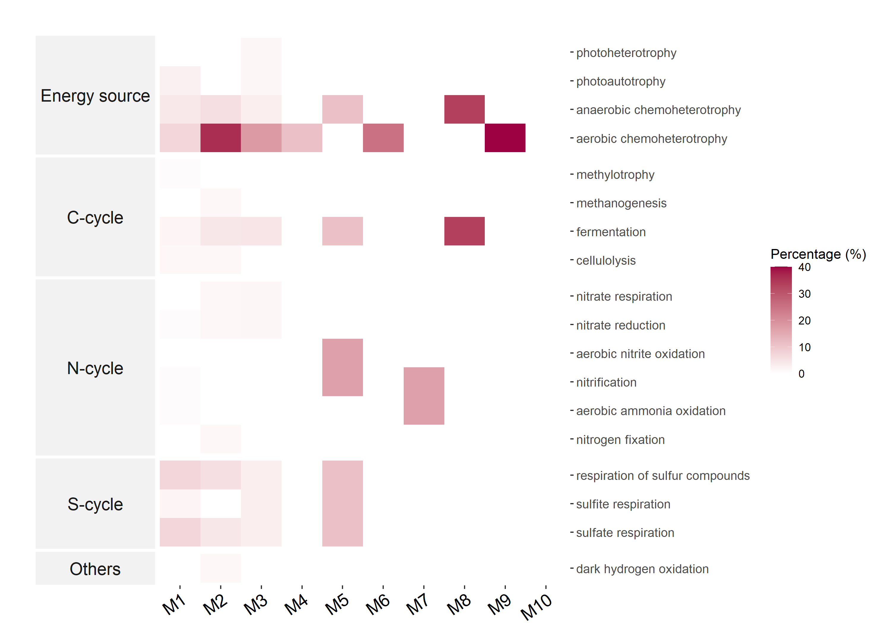
# If you want to change the group list, reset the list t2$func_group_list
t2$func_group_list
# use show_prok_func to see the detailed information of prokaryotic traits
t2$show_prok_func("methanotrophy")
Then we try to correlate the FR data in res_func_FR to environmental variables.
t3 <- trans_env$new(dataset = mt, add_data = env_data_16S[, 4:11])
t3$cal_cor(add_abund_table = t2$res_func_FR, cor_method = "spearman")
t3$plot_cor(cluster_ggplot = "both")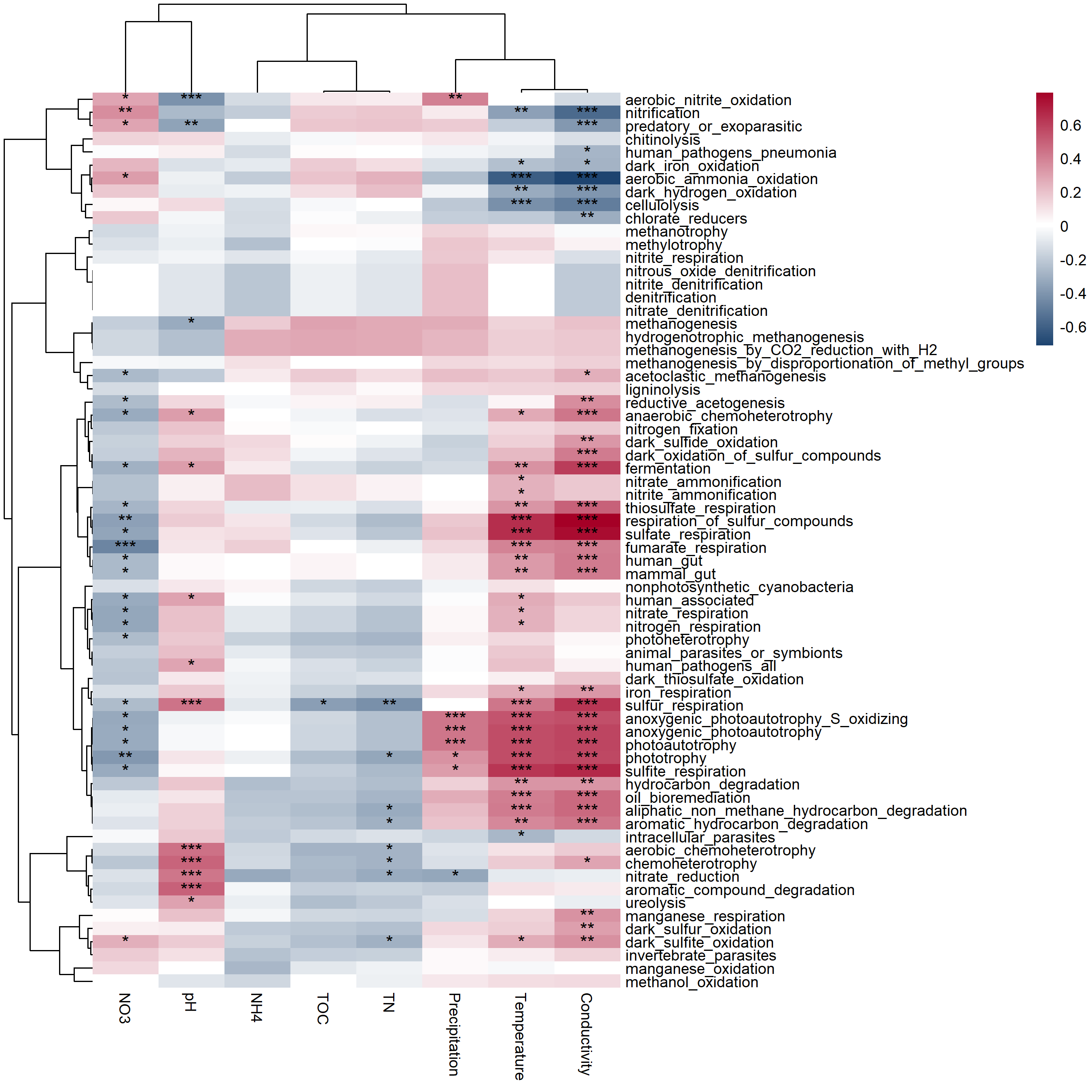
Tax4Fun2 (Wemheuer et al. 2020) is an R package for the prediction of functional profiles of prokaryotic communities from 16S rRNA gene sequences.
It also provides two indexes for the evaluation of functional gene redundancies.
If the user want to use Tax4Fun2 method, the representative fasta file is necessary to be added in the microtable object.
Please check out https://chiliubio.github.io/microeco_tutorial/intro.html#tax4fun2 to see
how to read fasta file with read.fasta of seqinr package or readDNAStringSet of Biostrings package.
Please also see https://chiliubio.github.io/microeco_tutorial/intro.html#tax4fun2 for downloading ncbi-blast and Ref99NR/Ref100NR.
For windows system, ncbi-blast-2.5.0+ is recommended since other versions can not operate well.
# load the example dataset from microeco package as there is a rep_fasta object in it
data(dataset)
dataset
# create a trans_func object
t1 <- trans_func$new(dataset)
# create a directory for result and log files
dir.create("test_prediction")
# https://chiliubio.github.io/microeco_tutorial/intro.html#tax4fun2 for installation
# ignore blast_tool_path parameter if blast tools have been in path
# the function can search whether blast tool directory is in the path, if not, automatically use provided blast_tool_path parameter
t1$cal_tax4fun2(blast_tool_path = "ncbi-blast-2.5.0+/bin", path_to_reference_data = "Tax4Fun2_ReferenceData_v2",
  database_mode = "Ref99NR", path_to_temp_folder = "test_prediction")

# calculate functional redundancies
t1$cal_tax4fun2_FRI()

# prepare feature table and metadata
data(Tax4Fun2_KEGG)
# create a microtable object for pathways
func_mt <- microtable$new(otu_table = t1$res_tax4fun2_pathway, tax_table = Tax4Fun2_KEGG$ptw_desc, sample_table = dataset$sample_table)
func_mt$tidy_dataset()
We further analyze the abundance of predicted metabolic pathways.
# calculate relative abundances at three levels: Level.1, Level.2, Level.3
func_mt$cal_abund()
print(func_mt)
Then, let’s use trans_abund class to visualize the abundance.
# bar plot at Level.1
tmp <- trans_abund$new(func_mt, taxrank = "Level.1", groupmean = "Group")
tmp$plot_bar(legend_text_italic = FALSE)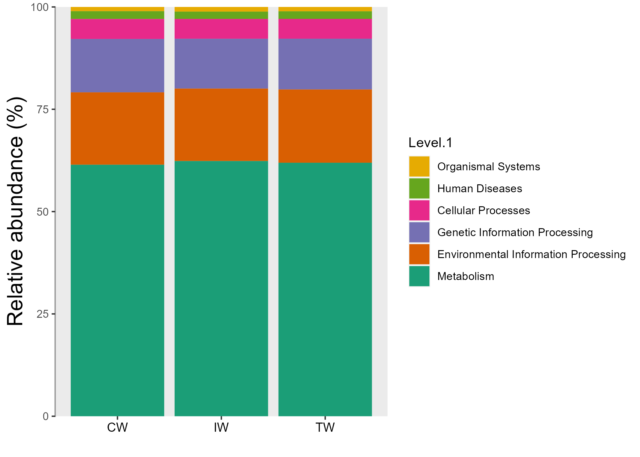
Then let’s perform the differential abundance test and find the important enriched pathways across groups.
tmp <- trans_diff$new(dataset = func_mt, method = "lefse", group = "Group", alpha = 0.05, lefse_subgroup = NULL)
tmp$plot_diff_bar(threshold = 3, width = 0.7)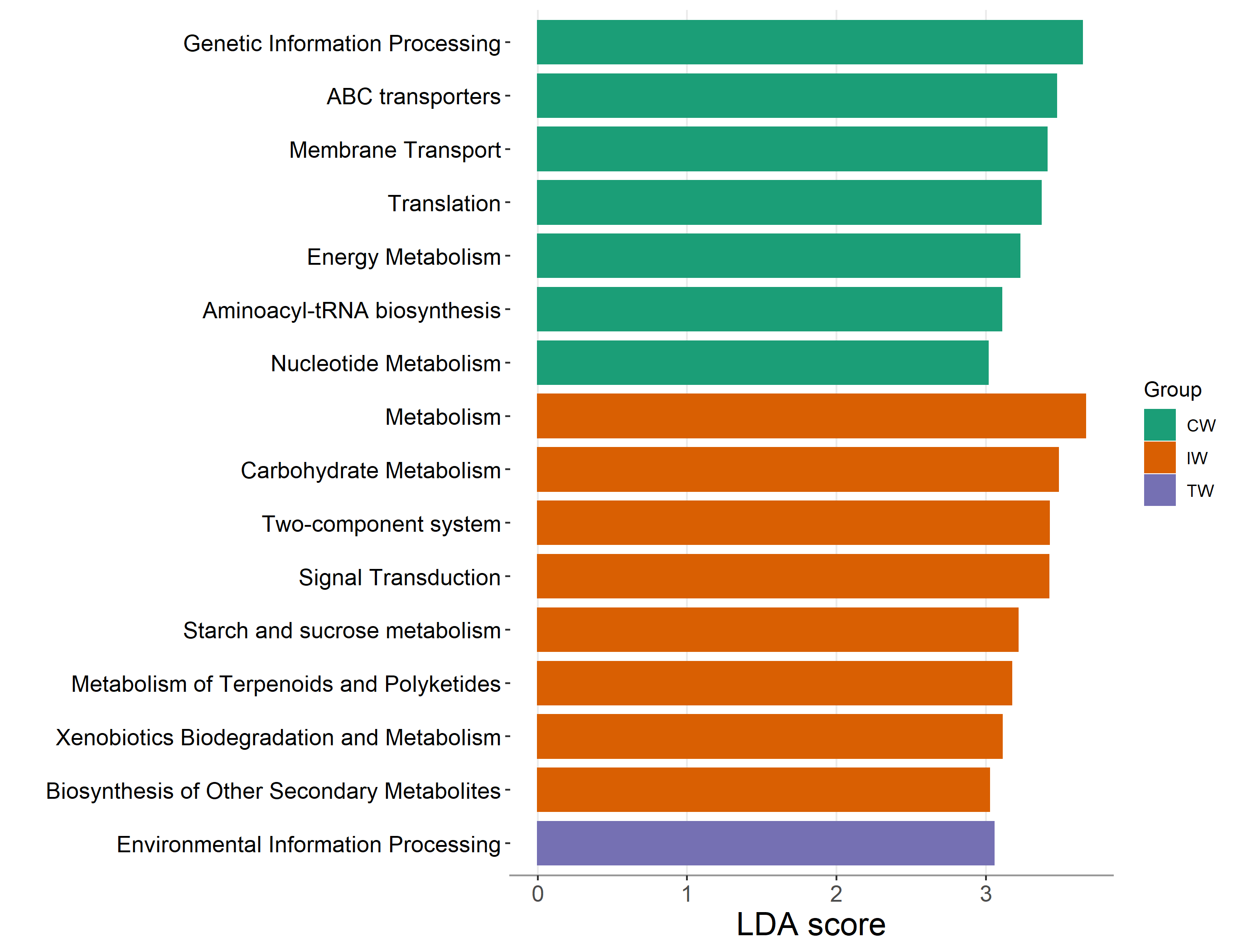
The subsequent analysis steps for PICRUSt2 (Douglas et al. 2020) are similar to those of Tax4Fun2. The main difference on operations between these two methods lies in the file reading part. PICRUSt2 requires reading the preliminary analysis result files. We have placed PICRUSt2 examples in the file2meco package section (https://chiliubio.github.io/microeco_tutorial/file2meco-package.html#picrust2).
7.2.2 Key points
- blast_tool_path parameter in cal_tax4fun2: if the blast tool has been in ‘environment variable’ of computer, it is ok to use blast_tool_path = NULL
- blast version: tax4fun2 require NCBI blast tool. However, some errors often come from the latest versions (https://www.biostars.org/p/413294/). An easy solution is to use previous version (such as v2.5.0).
7.3 trans_metab class
This class is a wrapper for a series of metabolite analysis, including origin inference (Wang et al. 2026) and pathway enrichment.
# use data inside the microeco package
tmp <- trans_metab$new(metab = soil_metab, microb = soil_microb)

# If the tax_table in the input metab data already contains detailed annotations (such as KEGG, HMDB columns),
# user can skip the following step. This step performs text-based matching to align the input metabolite names with those in the database.
# please download the database from https://zenodo.org/records/18618912; uncompress the zip file
# Fuzzy matching of metabolite names against those in the database
tmp$cal_match(database_path = "./metorigindb_split_202602")
# View(test$res_match)

# origin inference based on the database of TidyMass2
# The parameter match_col works by determining metabolite assignment based on the provided "names" (row names) or other columns (e.g., "KEGG_ID").
# For "names", the function first checks whether res_match (from the last step) exists; if it does, metabolite identification is performed according to the distance threshold.
tmp$cal_origin(database_path = "./metorigindb_split_202602", match_col = c("names", "HMDB_ID", "KEGG_ID"))
# tmp$res_origin_rawtable and tmp$res_origin_list

# create the metabolites-bacteria network according to the result from the last step
res_network <- tmp$cal_origin_network()

# use trans_network class to visualize the result
test <- trans_network$new()
test$res_network <- res_network
test$cal_module()
test$get_node_table()
head(test$res_node_table)

# test$plot_network(method = "networkD3", node_color = "type")


################################################
########## Pathway analysis
# Map metabolites to pathways based on a database
tmp$cal_pathway(db_type = "kegg")

# Perform pathway enrichment analysis for target metabolites using Fisher's exact test
target <- rownames(soil_metab$data_metab$otu_table)[1:50]
tmp$cal_pathway_enrich(target_metabs = target, p_adjust_method = "BH", p_cutoff = 0.05, min_metab_count = 3)

tmp$plot_pathway_enrich()


#### Following steps can be used to get the metabolite-pathway network
# res_net <- tmp$cal_pathway_network()

# test <- trans_network$new()
# test$res_network <- res_net
# test$cal_module()
# test$get_node_table()
# head(test$res_node_table)